Background

The dG0 timestep method (backward Euler) for the initial value problem

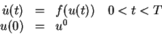$$\begin{array}{rcl} \dot u (t) &=& f(u(t)) \quad 0<t<T \\ u(0) &=& u^0 \end{array}$$ (1)

is, Find $U(t_n)$ successively for $n=1,\dots, N$ according to

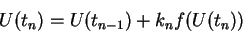$$U(t_n) = U(t_{n-1}) + k_n f(U(t_n))$$ (2)

The dual linearized problem is

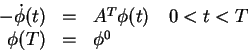$$\begin{array}{rcl} - \dot{\phi} (t) &=& A^T \phi(t) \quad 0<t<T \\ \phi(T) &=& \phi^0 \end{array}$$ (3)

where

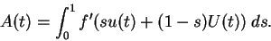$$A(t) = \int_0^1 f'(su(t) + (1-s)U(t))\: ds.$$ (4)

Note that the dual problem runs backward in time, starting at $t=T$. Replacing $u(t)$ by $U(t)$ gives the approximate formula for $A(t)$

$$A(t) \approx f'(U(t))$$ (5)

An adaptive scheme for solving the IVP could be formulated as, choose an appropriate step length $k_n$ such that

$$k_n = \frac{\textrm{TOL}}{S_c(t)\cdot R_n}$$ (6)

where $\textrm{TOL}$ is your error tolerance, $S_c(t)$ the stability factor defined by

$$S_c(t) = \frac{\int_0^T \Vert \dot \phi(s)\Vert \: ds} {\Vert\phi_0\Vert},$$ (7)

where $\phi$ solves (3). $R_n$ is the residual. A more useful approximation is to use $R_{n-1}$ instead of $R_n$.